How to efficiently prewhiten fMRI timeseries the “right” way

I recently got around to reading the high-profile PNAS paper titled “Cluster failure: Why fMRI inferences for spatial extent have inflated false-positive rates” (Eklund et al. 2016), which called attention to the importance of properly processing and analyzing fMRI data.

This lead me to an earlier paper titled “Does parametric fMRI analysis with SPM yield valid results?” (Eklund et al. 2012), which identified mismodeling of temporal autocorrelation as a major factor driving high false positive rates.  From a statistical perspective, accounting for temporal autocorrelation is vital to obtain correct standard errors on model coefficients, which are the basis for hypothesis tests used to identify areas of activation in the brain, a primary goal in many fMRI studies.  (In fact many group analyses actually ignore first-level standard errors, but these should ideally be incorporated into the second-level model.)

The 2012 paper pointed out two primary reasons for mismodeling of temporal autocorrelation: (a) using too low of a model order, such as AR(1), especially for faster TRs, and (b) assuming the same AR coefficients across the brain.  They also recommend smoothing the coefficients to improve the estimates.

As a statistician, I was excited to try out this “proper” approach to prewhitening.  Increasing the model order was no big deal (I used an AR(6) model for TR=0.72 seconds), but doing the prewhitening at the voxel level was a bit of a hassle.  After much trial and error and a few new gray hairs, here’s what I’ve learned.  Some of the computational strategies are specific to R, but they can probably be easily adapted to MATLAB or Python.

1. AR coefficients definitely seem to vary across the brain.
2. Averaging across subjects greatly improves the smoothness of the coefficient maps, which is presumably indicative of better estimation.
3. The prewhitening matrix (the square root inverse covariance matrix) needs to be computed quickly, since you’re going to be doing it separately for every voxel in the brain.

I’ll go into each of these in turn below, but first, let’s review why and how prewhitening is actually performed.  fMRI task activation studies typically rely on fitting a regression model at many different locations in the brain, and ordinary least squares regression assumes uncorrelated errors.  This assumption is the basis of how we compute standard errors of coefficient estimates, which in turn are the basis of hypothesis testing, which allows us to identify regions of the brain that are active in response to different tasks.  The validity of these hypothesis tests depends primarily on (1) how correction for multiple comparisons was performed (the focus of the 2016 paper mentioned above) and (2) the accuracy of the standard errors of the model coefficients.  If we ignore temporal autocorrelation, we will underestimate the true standard errors and obtain more false positives.

So how do we fix this?  If y (T×1) is the time series for a single voxel and X (T×k) is the design matrix containing an intercept, column(s) corresponding to the expected BOLD response under the task paradigm, and several columns for nuisance parameters such as motion and drift, then the regression model we want to estimate is y = Xβ + ε, where ε ~ Normal(0, σ²V).  The β coefficients corresponding to the task-related columns of X represent the level of activation in response to each task at this particular voxel.  V is a T×T temporal correlation matrix.  If we knew V, then we could simply pre-multiply both sides of the equation by W=V^-1/2, since Wy = WXβ + Wε, where Wε has variance/covariance matrix σ²WVW=σ²I.  Ideally this should be done several times, pre-multiplying again by the new W at each iteration.  This results in a regression model with uncorrelated errors, which we can fit as usual to obtain estimates and valid standard errors for β.

So how do we find W?  We first solve the original regression equation y = Xβ + ε to get an estimate of the residuals, then fit an AR(p) model to the residuals to get the p AR coefficient estimates.  We can then compute V^-1 directly (it has a simple form, see point 3 below), then take its square root to get W.  Simple enough.

The challenge is how to do this for every voxel in the brain and every subject in our analysis without it presenting a major computational inconvenience.  If we intend to average the coefficients across our n subjects (which we probably should – see point 2 below), then our work flow should look like:

(a) estimate the p AR coefficients for each location in the brain and each subject (resulting in a total of p*n images)

(b) average them across subjects (resulting in a total of p images)

(c) compute the prewhitening matrix W for each location in the brain (resulting in N T×T matrices, where N is the number of voxels in the brain), and

(d) fit the regression model Wy = WXβ + Wε at each voxel to get estimates and standard errors for β for each subject and voxel, which can then be passed on to a group-level model.

If this sounds like a lot of work, here’s several reasons to do it anyway:

1. AR coefficients vary across the brain.

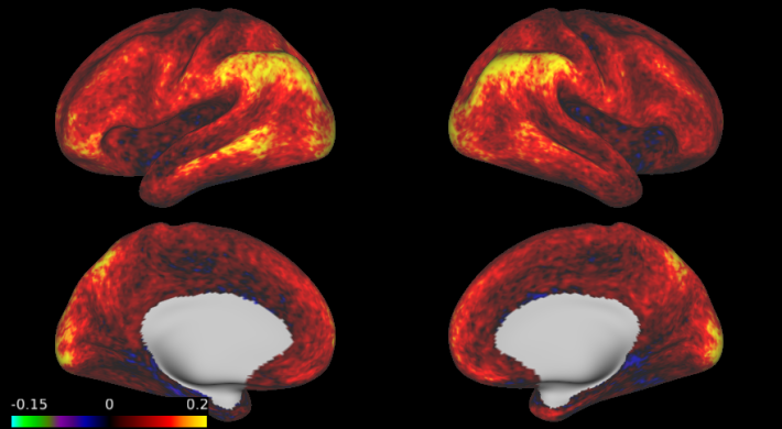
For my AR(6) model fit on motor task data from the Human Connectome Project, here are the estimates of the AR coefficients (from a single iteration), averaged across ~500 subjects.  Each image is on a different scale, since the magnitude of the coefficients tends to decrease with the time lag.  However, what is shared across the coefficients is the fact that there are striking spatial variations.  And the spatial differences are not minor – the first coefficient varies from nearly zero in the medial temporal lobe (MTL) to over 0.2 in the angular gyrus and occipital cortex, while the second coefficient is largely positive but with some areas of negative autocorrelation in the MTL and the inferior frontal cortex.

2. Efficiency of coefficient estimates can be improved by averaging across subjects.

[The term “efficiency” in the title of this post has a double meaning: estimation efficiency has to do with obtaining estimates that have low variance, meaning they are close to the truth (assuming they are unbiased), while computational efficiency (see point 3) is the ability to compute stuff quickly.  Both are important, but for very different reasons.  Estimation efficiency matters because it influences accuracy of “activated regions”; computational efficiency matters because time is scarce.]

For the same AR(6) model, here are the estimates of the first AR coefficient averaged across 500 subjects, 20 subjects, and for a single subject.  The averaged images are much smoother than the single-subject image.  Another option would be to perform a small amount of spatial smoothing, especially if you want to allow for differences across subjects.

3. The prewhitening matrix can be computed quickly for each voxel.

Hopefully you’re now convinced that voxel-wise prewhitening and averaging coefficient estimate across subjects is important.  But if it takes weeks to run and debug, let’s get real – it’s probably not going to happen. Luckily, each of the four steps in the workflow can be done reasonably quickly:

(a) Estimate the p AR coefficients for each location in the brain and each subject.  Instead of looping through all voxels to obtain residuals, this can be done very quickly by keeping everything in matrix form.  Letting Y be the T×V matrix of voxel time series, then B = (X’X)^-1X’Y is the k×V matrix of coefficient estimates, and E = Y – XB is the T×V matrix of residuals.  Then you just need to loop over voxels to fit an AR model to each column of E.

(b) Average the coefficients across subjects. Sum and divide by n.

(c) Compute the prewhitening matrix W for each location in the brain. I chose to do this by looping through voxels and computing W for each voxel.  This means that for each voxel, you’ll end up computing the same W n times, once for each subject.  Alternatively, the N different prewhitening matrices (one for each voxel) can be computed once and stored, which can be done efficiently using sparse matrices with the Matrix package in R.  But actually W can be computed very quickly, so it’s no big deal to do it on the fly.

To compute W, you first need to compute V^-1.  For an AR(p) model with coefficients φ₁, …,φ_p, V^-1 is (proportional to) AA^t, where A is a banded diagonal matrix with 1’s on the main diagonal, -φ₁ on the first lower off-diagonal, -φ₂ on the second lower off-diagonal, etc., and zeros everywhere else (including the entire upper triangle).  (You might notice that the main diagonal of the resulting V^-1 has all its elements equal except for the first p and last p elements.  This is a boundary effect due to fitting an AR(p) model with fewer than p time points at the beginning and end of the timeseries.  The first p time points of W, y and X should therefore be discarded prior to model fitting.)

Once you have V^-1, perform singular value decomposition or compute its eigenvalues U and eigenvectors d to write V^-1=UDU^t, where D=diag{d}.  Then W is simply V^-1/2=UD^1/2U^t.  This takes about 0.2 seconds, compared with about 30 seconds using the sqrtm() function in R.

(d) Fit the regression model Wy = WXβ + Wε at each voxel.  Here it’s probably easiest just to loop through, since W and therefore WX are different for each voxel, so the matrix-based approach used in (a) no longer works.  Since W is fast to compute, this isn’t so bad.

That’s about it!  If you have an experience or perspective to share, please add them in the comments.  I would love to hear your thoughts.